Description of TFIT
TFIT (Laidler et al. 2007) was initially conceived and written by C. Papovich in 1999 as a C++ code.In its latest version, TFIT consists of a Python envelop performing the entirety of tasks, except for the fitting core routine, which is based on the original C++ routines. It requires the pre‐ installation of the following software: Python (and some of its standard modules/interfaces, such as numpy, scipy, matplotlib, anfft, pyraf); CFITSIO libraries; STSCI; IRAF; STSDAS; FFTW3.
The HRI and the LRI must be aligned and their pixel scales must be the same or have integer ratio (these requirements can be accomplished for example using SWARP, Bertin et al. 2002, and/or the IRAF tasks CCMAP and SREGISTER).
TFIT can subtract a constant background (given in the input catalog), but it is instead recommended to perform a detailed background subtraction before running TFIT, thus putting the term B equal to zero in the linear system to be solved.
The preliminary steps (cutting out of priors and their convolution with the kernel) are performed in “stages”, in which all sources are processed before passing at the following step. The cutout stage is performed invoking the IRAF task imcopy, via pyraf call. The convolution stage is performed using a Fast Fourier Transform routine (FFTW3), invoked via the anfft Python module (in TFIT original release, the convolution was instead performed via straight pixel-‐by-‐pixel summation). Cutouts and templates are stored as FITS files, generally requiring quite a large amount of memory.
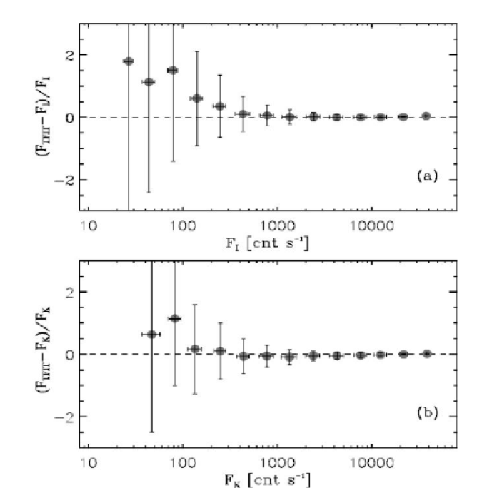
Comparison between the SExtractor isophotal flux (FI; top) and the SExtractor Kronlike flux (FK; bottom) from the high-‐resolution image vs. the flux derived by TFIT from the low-‐resolution images for ≈1300 sources in a simulated images. (a) Flux difference, (FLRI Ϫ FI)/FI , vs. isophotal flux from the high-‐resolution image. The sources have been binned in intervals of quarter magnitudes, and the error bars indicate the standard deviation for the sources in that bin. For this simulation, the standard error in the mean is one-‐tenth the standard deviation. (b) Same as (a), except TFIT fluxes are compared to the Kronlike fluxes of SExtractor.
In TFIT the linear system is not built on the LRI as a whole at once. Rather, the LRI is divided into an arbitrary grid of “cells”, and a linear system is built and solved for each of these cells. The typical dimension of a cell should be more than say 30 times the LRI FWHM (a wrong choice of the cell dimension may lead to catastrophic errors); the grid is constructed in such a way that cells overlap, and each cell is then expanded once to completely contain the sources which partly fell into its original dimensions. Moreover, a second fitting run is performed using a shifted (dithered) grid. In this way, each source is fitted more than once (usually at least 4 times for a standard choice of the dimensions of cells). At the end of the fitting procedure, the “best choice” for each source is selected picking the fit obtained within the cell in which the object is at the minimal distance from the geometrical center.
This method strongly reduces the computational time, because the solution of a very large sparse linear system is usually computationally far more expensive than the solution of a large number of small ones. On the other hand, it introduces some degrees of arbitrariness in the procedure, which may lead to systematic inaccuracies in the determination of the fluxes. Further analysis is being performed on the issue.
The linear system solution is performed by the C++ core code, via LU decomposition of the matrix (in the TFIT original version, the Singular Value Decomposition method was adopted instead). No constraint is imposed on the fitting constants, so negative fluxes can be found and kept as “right” solutions.
Diagnostics and error estimates are also computed during this stage, and outputted both numerically and graphically (i.e., covariance matrix -‐ whose diagonal consists of the squares of the errors to be assigned to each source -‐ and residual images).
After the first fitting procedure is completed, a “collage model image” is constructed using the templates, each multiplied by its fitting constant. Then, each region of the LRI is cross-‐ correlated with the corresponding region of this collage image, and the resulting “best fitting shifts” in x and y are found. Finally, a set of shifted convolution kernels which maximize the correlation for each region are produced. All of these procedures are performed invoking IRAF tasks, namely xregister and imlintran.
The stages of convolution and fitting are then repeated from scratch, this time degrading each HRI cutout using the new “shifted” convolution kernel found for the region of the LRI to which it belongs. In this way, a higher degree of precision is obtained in the astrometry registration of each source.
A complete (double) run on a standard astronomical field (say, one Goods-‐S Hawk-‐I field) requires ca. 48 hours on a standard machine, this estimate strongly varying depending on the number of sources in the HRI catalog falling outside the LRI (these are cut and convolved anyway, and later excluded from the minimization procedure). This long executing time is largely due to the slowness of the Python procedures.
TFIT is currently being reviewed and improved, and a new version is expected to be released in the next months.